6 Post-Selection Inference

6.1 Introduction

When model selection is performed with the intention to use the selected model for inference (not only prediction), i.e. for a better understanding of the phenomenon under study, one needs inferential methods (e.g. building confidence intervals, testing) that take account the variability induced by data-based model selection methods. In other words, by ignoring the variability introduced by the model selection step, one introduces biases when computing for example confidence intervals for slope coefficients in the linear regression model. The bias always lowers the risk measure (variance) estimator, resulting in smaller confidence intervals and possibly also not centered around the true values. This can have important impacts when for example evaluating the strength of a drug (dosage) on an health-related outcome.

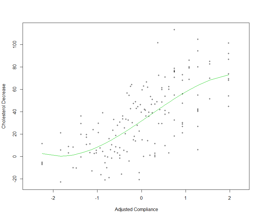
As an illustrative example, consider the data set cholesterol analysed in Efron and Hastie (2016) which concerns the response of 164 men to a treatment (over a period of 7 years) for lowering cholesterol levels in the body. The single predictor is a (standardized) fraction of intended dose (of the cholesterol lowering drug cholestyramine) actually taken (compliance). The response is the decrease in cholesterol level over the course of the experiment. A potential suitable model (or family of models) for the relationship between the decrease of the cholesterol level and the amount of cholestryramine (compliance) is a polynomial regression model \[\begin{equation} \boldsymbol{Y}=\sum_{j=0}^J\beta_jX^j+\boldsymbol{\varepsilon}=\beta_0+ \beta_1X+\beta_2X^2+\ldots +\beta_JX^J+\boldsymbol{\varepsilon} \end{equation}\]

A model selection method is typically applied here to select \(J\). For the cholesterol data, using the \(C_p\) as model selection criterion (note that the sequence of ordered models is given), provides \(J=3\) as the best model.

Polynomial fit (\(J=3\)) for the cholesterol data

With this example, one might be interested in building a confidence interval for the response to treatment, at a given treatment level \(X\). Letting \(\mu=\sum_{j=0}^J\beta_jX^j\), one actually seeks a confidence interval \(CI_{1-\alpha}\left(\mu\vert \hat{\boldsymbol{\beta}},\hat{J}\right)\) constructed from the sample via \(\hat{\boldsymbol{\beta}}\) and \(\hat{J}\). Ignoring the randomness of \(\hat{J}\) (i.e. by fixing \(J=\hat{J}\)) and performing standard inference using \(\hat{\mu}=\sum_{j=0}^J\hat{\beta}_j\mathbf{x}^j\) will provide misleading confidence intervals.

6.2 Inference via the nonparametric Bootstrap

One way to infer (computing confidence intervals) is by reproducing simultaneously the selection and estimation mechanism by means of the nonparametric bootstrap: \(B\) samples of size \(n\), \(\left(y_i^b,x_i^b\right), i=1,\ldots,n\), are created by drawing with replacement from the original sample. On each of the \(B\) samples, selection (using e.g. the \(C_p\)) is performed to obtain \(\hat{J}^b\), estimates \(\hat{\beta}_j^b\) used in computing \(\hat{\mu}^b=\sum_{j=0}^{\hat{J}^b}\hat{\beta}_j^b\mathbf{x}^j\). The Figure below provides the bootstrap distribution of \(\hat{\mu}^b\), for a compliance \(x=-2\), and for \(\widetilde{\mu}^b=\sum_{j=0}^{J}\hat{\beta}_j^b\mathbf{x}^j\) with \(J=3\), the value found in the original sample.

Bootstrap distribution of \(\tilde{\mu}^b\) (fixed) and \(\hat{\mu}^b\) (adaptive) on the cholesterol data

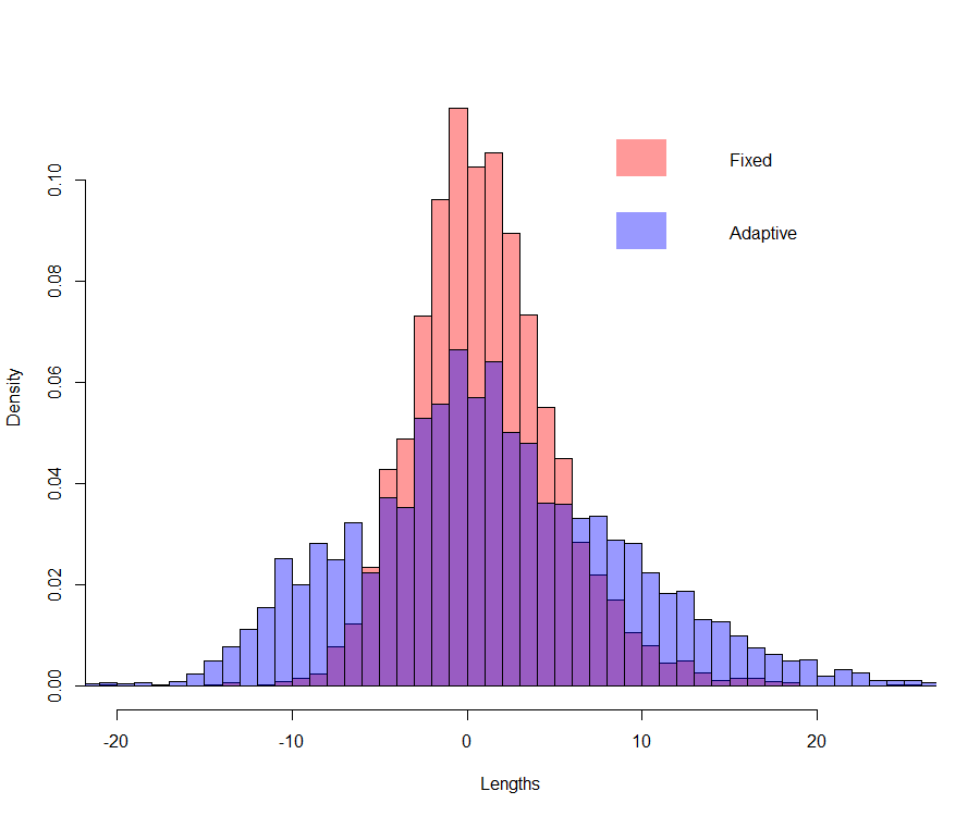
As expected, the length of the confidence intervals are underestimated when one ignores the randomness introduced by the selection procedure (i.e. the randomness of \(\hat{J}\)). Actually, the confidence interval for \(\mu\) at \(x=-2\) (estimated via the nonparametric bootstrap) ignoring the randomness of the selection procedure is \(CI_{1-\alpha}\left(\mu\vert J=3\right)=1.05 \pm 8.09\) while not ignoring the randomness of the model selection procedure it is \(CI_{1-\alpha}\left(\mu\vert \hat{J}=3\right)=1.40 \pm 16.17\).

What actually happens with (hard thresholding) model selection criteria such as the \(C_p\) is that it is a discontinuous process, creating jumps in the estimates. In the cholesterol data example, with the nonparametric bootstrap, for about \(20\)% of the bootstrap samples, the \(C_p\) selected \(\hat{J}=1\), i.e. the linear model. In these cases, \(\hat{\mu}^b\vert \hat{J}=1\) are smaller. This is illustrated in the Figure below.

Bootstrap distribution of \(\tilde{\mu}^b\) (Fixed: \(J=3\)), \(\hat{\mu}^b\vert \hat{J}=1\) (Adaptive: \(J=1\)) and \(\hat{\mu}^b\vert \hat{J}>1\) (Adaptive: \(J>1\)) on the cholesterol data

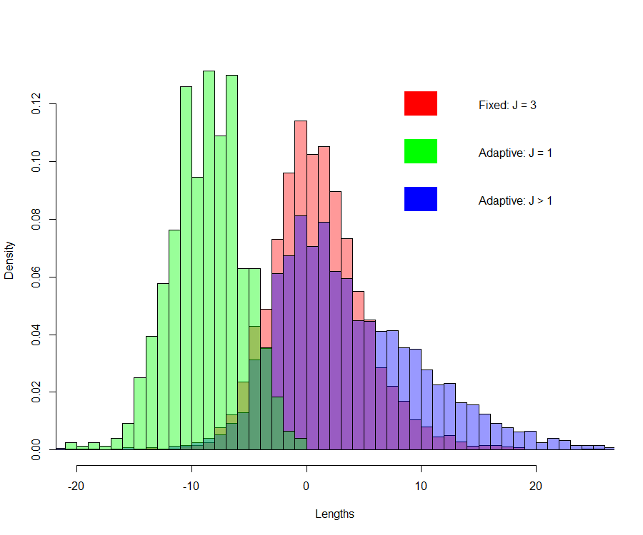
The distribution of the \(\hat{\mu}^b\) when \(\hat{J}=1\) is clearly different (different location) that the distribution of the \(\hat{\mu}^b\) when \(\hat{J}>1\). \(\hat{J}=1\) happens in about 20% of the bootstrap samples, which creates, from one sample to the other, important jumps.

6.3 Improving on the Bootstrap: Smoothed Bootstrap or Bagging

Bagging stands for bootstrap averaging and leads to "improvements for unstable procedures" (Breiman 1996), which include subset selection in linear regression (Breiman 1994). Bagging is also known as bootstrap smoothing (Efron and Tibshirani 1996). Given bootstrap replicates of a bootstrapped statistic \(T^b, b=1,\ldots,B\), the bootstrap standard errors are computed using the bootstrap distribution as \[\begin{equation} \widehat{\mbox{sd}}_B=\sqrt{\frac{1}{B-1}\sum_{b=1}^B\left(T^b-\overline{T}_B\right)^2} \end{equation}\] with \[\begin{equation} \overline{T}_B = \frac{1}{B}\sum_{b=1}^BT^b \end{equation}\]

Since after a bootstrap sampling, \(\overline{T}_B\) is available, the bagging method proposes to compute the standard errors associated to \(\overline{T}_B\), which are lower. A brute force method would bootstrap several values for \(\overline{T}_B\) which ends up in large computational times and is prohibitive in high dimensions. Actually, there is no need to resample further.

Let \(N_{bi}\) denote the number of times observation \(i\) occurs in the bootstrap sample \(b\). The vector \(\mathbf{N}_b=\left(N_{1b},\ldots,N_{nb}\right)\) has a multinomial distribution with \(n\) draws on \(n\) categories each with associated probability \(1/n\), and has mean vector and covariance matrix \[\begin{equation} \mathbf{N}_b \sim \mbox{Mult}\left(\boldsymbol{1}_n, \mathbf{I}_n-\frac{1}{n}\boldsymbol{1}_n\boldsymbol{1}_n\right) \end{equation}\] with \(\boldsymbol{1}_n\) the \(n\times 1\) vector ones. Using this setting, Efron (2014) shows that the infinitesimal jackknife estimate of the standard deviation for \(\overline{T}_B\) is \[\begin{equation} \sqrt{\sum_{i=1}^n\mbox{cov}^2\left(N_{bi},T^b\right)} \end{equation}\] A suitable estimator is given by \[\begin{equation} \widetilde{\mbox{sd}}_B=\sqrt{\sum_{i=1}^n\widehat{\mbox{cov}}^2\left(N_{bi},T^b\right)} \end{equation}\] with \[\begin{equation} \widehat{\mbox{cov}}^2\left(N_{bi},T^b\right)=\frac{1}{B}\sum_{b=1}^B\left(N_{bi}-N_{\cdot i}\right)\left(T^b-\overline{T}_B\right) \end{equation}\] and \(N_{\cdot i}=(1/B)\sum_{b=1}^BN_{bi}\). Moreover, it is always true that \[\begin{equation} \frac{\widetilde{\mbox{sd}}_B}{\widehat{\mbox{sd}}_B}\leq 1 \end{equation}\]

Bagging with the infinitesimal jackknife allows to be more precise than with the bootstrap without the need to simulate (bootstrap) more replicates, which makes it a computationally convenient inferential method. For the cholesterol data example, the standard deviations (across values for \(x\)) decrease of about 12%. In general, the savings due to bagging increase with the nonlinearity of \(T^b\) and is therefore a suitable approach for inference after selection. Wager, Hastie, and Efron (2014) have used this approach to derive confidence intervals for Random Forests. Bagging is actually a form of model averaging.

6.4 Universally valid POst-Selection Inference (PoSI)

Quite recently, test statistics and their associated distribution have been proposed in the linear regression case, to test hypothesis about slope parameters, that take into account the randomness of the selection part of the analysis. It is actually possible to formalize the conditional distribution of (a linear combination of) the slope estimators (typically the LS), conditionally on the distribution of the outcome of the selection method. The quantiles of the conditional distribution are then obtained by Monte-Carlo simulations. The material in this section is taken form Zhang, Khalili, and Asgharian (2022).

Let define the projection-based regression coefficients corresponding to a given submodel \(\cal{M}\) as \[\begin{equation} \mathbf{b}_{\cal{M}} = \text{argmin}_{\mathbf{b}}\Vert\mu −\mathbf{X}_{\cal{M}}\mathbf{b}\Vert^2 = \left(\mathbf{X}_{\cal{M}}^T\mathbf{X}_{\cal{M}}\right)^{-1}\mathbf{X}_{\cal{M}}\boldsymbol{\mu} \end{equation}\]

where \(\boldsymbol{\mu}=\mathbb{E}[\mathbf{Y}\vert\mathbf{X}_{\cal{M}_{\small \text{all}}}]\). Berk et al. (2013) propose the so-called PoSI method, which is capable of producing universally valid post-selection confidence intervals for the projection-based regression coefficients \(b_{j,\widehat{\cal{M}}}, j \in \widehat{\cal{M}}\), regardless of model selection procedures and selected submodel \(\widehat{\cal{M}}\). Here “valid” means the confidence intervals achieve at least the nominal coverage probability \(1−\alpha\),for any \(\alpha \in (0, 1)\), by taking into account the model selection stage. The merit of the PoSI method is that even if a selected submodel deviates from the true model, it still guarantees valid inference for that selected submodel.

More precisely, given a submodel \(\widehat{\cal{M}}\in \cal{M}_{\small\text{all}}\) selected by a generic model selection procedure, the confidence interval for \(b_{j,\widehat{\cal{M}}}\) is generally given by \[\begin{equation} CI_{j,\widehat{\cal{M}}}(K) = \left(\hat{\beta}_{j,\widehat{\cal{M}}}-K\cdot \hat{\sigma}\left[\left(\mathbf{X}_{\widehat{\cal{M}}}^T\mathbf{X}_{\widehat{\cal{M}}}\right)^{-1}\right]_{jj}; \hat{\beta}_{j,\widehat{\cal{M}}}+K\cdot \hat{\sigma}\left[\left(\mathbf{X}_{\widehat{\cal{M}}}^T\mathbf{X}_{\widehat{\cal{M}}}\right)^{-1}\right]_{jj} \right) \end{equation}\]

where \(\hat{\beta}_{j,\widehat{\cal{M}}}\) is the OLS at model \(\widehat{\cal{M}}\), \(\hat{\sigma}^2\) is the estimated error's variance at the full model and \(K\) is a scalar that needs to be estimated. If \(K\) is replaced by the quantile \(1-\alpha/2\) of the \(t\)-distribution with \(n-\vert\widehat{\cal{M}}\vert\) degrees of freedom, we obtain the naıve confidence interval, which does not have the proper coverage (far more liberal).

The goal of the PoSI approach is hence to have a potentially larger value of the constant \(K\) to capture the extra randomness brought about by data-dependent model selector. In this way, the resulting confidence interval becomes wider and thus capable of achieving the nominal coverage probability, regardless of model selection procedures and selected submodels. This objective can be achieved by choosing the constant \(K\), for a given significan level \(1-\alpha\), that satisfies \[\begin{equation} P\left(b_{j,\widehat{\cal{M}}}\in CI_{j,\widehat{\cal{M}}}(K), \forall j \in \widehat{\cal{M}}\right)\geq 1 − \alpha, \alpha \in (0, 1). \end{equation}\] Berk et al. (2013) show that \(K\) also satisfies \[\begin{equation} P\left(\text{max}_{j}\vert t_{j,\widehat{\cal{M}}}\vert\leq K\right)\geq 1-\alpha \end{equation}\] with \[\begin{equation} t_{j,\widehat{\cal{M}}}=\frac{\mathbf{e}_j\left(\mathbf{X}_{\widehat{\cal{M}}}^T\mathbf{X}_{\widehat{\cal{M}}}\right)^{-1}\mathbf{X}_{\widehat{\cal{M}}}\boldsymbol{\varepsilon}} {\hat{\sigma}\left[\left(\mathbf{X}_{\widehat{\cal{M}}}^T\mathbf{X}_{\widehat{\cal{M}}}\right)^{-1}\right]_{jj}^{1/2}} \end{equation}\]

where \(\mathbf{e}_j\) is the \(j\)th standard basis (i.e. a vector of \(0\) expect a \(1\) at the \(j\)th element) and \(\boldsymbol{\varepsilon}\) is the random error. The constant \(k\) is actually the \(100(1 − \alpha/2)\)th percentile of the distribution of \(T=\text{max}_jt_{j,\widehat{\cal{M}}}\) which can be approximated using Monte Carlo simulations. Specifically, the Monte Carlo copies of T are based on independent draws of \(\boldsymbol{\varepsilon}\), with \(\varepsilon_i\sim \mathcal{N}(0, \sigma^2)\), with \(\sigma^2\) estimated by the residual variance at the full model. This computation has been implemented in the R package PoSI (Buja and Zhang (2015)).

Alternatively, Lee and Taylor (2014) and Lee et al. (2016) present an approach which depends on the model selection procedure and the selected submodel. Specifically, they construct confidence intervals with the exact \((1 − \alpha)\) coverage probability via conditioning on a selected submodel. The central point of this approach, i.e. the conditionally Exact POst-Selection Inference (EPoSI) approach is the determination of the conditional distribution of \(\left(\hat{\beta}_{j,\cal{M}}\vert \widehat{\cal{M}}=\cal{M}\right)\) which turns out to be a truncated normal distribution. For the later, an important result is provided by the polyhedral lemma or polyhedral selection property. Examples of model selection procedures having this property include, but not limited to, LASSO and elastic net with fixed tuning parameters, marginal screening and orthogonal matching pursuit. More detailed information can be found in Zhang, Khalili, and Asgharian (2022).

References

Berk, R., L. Brown, A. Buja, K. Zhang, and L. Zhao. 2013. “Valid Post-Selection Inference.” The Annals of Statistics 41: 802–37.

Breiman, L. 1994. “Bagging Predictors.” Technical Report 421. Department of Statistics, University of California, Berkeley.

Breiman, L. 1996. “Bagging Predictors.” Machine Learning 24: 123–40.

Buja, A., and K. Zhang. 2015. “PoSI: Valid Post-Selection Inference for Linear LS Regression.” R Package.

Efron, B. 2014. “Estimation and Accuracy After Model Selection.” Journal of the American Statistical Association 109: 991–1007.

Efron, B., and T. Hastie. 2016. Computer Age Statistical Inference: Algorithms, Evidence, and Data Science. Cambridge University Press.

Efron, B., and R. Tibshirani. 1996. “Using Specially Designed Exponential Families for Density Estimation.” Annals of Statististics 24: 2431–61.

Lee, J. D., D. L. Sun, Y. Sun, and J. E. Taylor. 2016. “Exact Post-Selection Inference, with Application to the Lasso.” The Annals of Statistics 44: 907–27.

Lee, J., and J. Taylor. 2014. “Exact Post Model Selection Inference for Marginal Screening.” Advances in Neural Information Processing Systems 27: 136–44.

Wager, S., T. Hastie, and B. Efron. 2014. “Confidence Intervals for Random Forests: The Jackknife and the Infinitesimal Jackknife.” Journal of Machine Learning Research 15: 1625–51.

Zhang, D., A. Khalili, and M. Asgharian. 2022. “Post-Model-Selection Inference in Linear Regression Models: An Integrated Review.” Statistics Surveys 16: 86–136.