4 Shrinkage Methods

4.1 Introduction

Shrinkage methods denote estimation methods under constraints that shrink estimators toward a given value. The origin goes back to the James–Stein estimator (James and Stein 1961). The rationale is that one can sacrifice bias for variance, i.e. optimize in some sense the Mean Squared Error (MSE), which, for an estimator \(\hat{\boldsymbol{\beta}}\) is \[\begin{equation} \mbox{MSE}\left(\hat{\boldsymbol{\beta}}\right)=\mathbb{E}\left[\left\Vert\hat{\boldsymbol{\beta}}-\boldsymbol{\beta}\right\Vert^2\right]=\mathbb{E}\left[\left(\hat{\boldsymbol{\beta}}-\boldsymbol{\beta}\right)^T\left(\hat{\boldsymbol{\beta}}-\boldsymbol{\beta}\right)\right] \end{equation}\]

(see Efron and Hastie (2016), Section 7.1, for details on the James–Stein estimator)

For the least squares (LS) estimator of the linear model \(\mathbf{y}=\mathbf{X}\boldsymbol{\beta}+\boldsymbol{\varepsilon}\), \(\boldsymbol{\varepsilon}\sim N\left(\mathbf{0},\sigma^2\mathbf{I}\right)\), and supposing without loss of generality that \(\mathbf{y}\) is centered and the covariates (columns in \(\mathbf{X}\)) are standardized, we have \(\mbox{MSE}\left(\hat{\boldsymbol{\beta}}_{LS}\right)=\sigma^2\mbox{tr}\left[\left(\mathbf{X}^T\mathbf{X}\right)^{-1}\right]\), which obviously grows with the dimension \(p\).

In terms of out-of-sample prediction error (PE), we have the following result \[\begin{eqnarray} \mbox{PE}\left(\mathbf{x}_0,\hat{\boldsymbol{\beta}}\right) &=&\sigma^2+\mathbb{E}_{Y\vert\mathbf{X}=\mathbf{x}_0}\left[\left(Y-\mathbf{x}_0\hat{\boldsymbol{\beta}}\right)\right]^2 +\mathbb{E}_{Y\vert \mathbf{X}=\mathbf{x}_0}\left[\left(Y-\mathbf{x}_0\hat{\boldsymbol{\beta}}\right)^2\right] \\ &=& \sigma^2+\mbox{Bias}^2\left(\mathbf{x}_0,\hat{\boldsymbol{\beta}}\right)+ \mbox{var}\left(\mathbf{x}_0,\hat{\boldsymbol{\beta}}\right) \end{eqnarray}\]

As model becomes more complex (more terms included), on one hand, local structure/curvature can be picked up, but on the other hand, coefficient estimates suffer from high variance as more terms are included in the model (see overfitting phenomenon).

Reported from http://statweb.stanford.edu/~tibs/sta305files/Rudyregularization.pdf

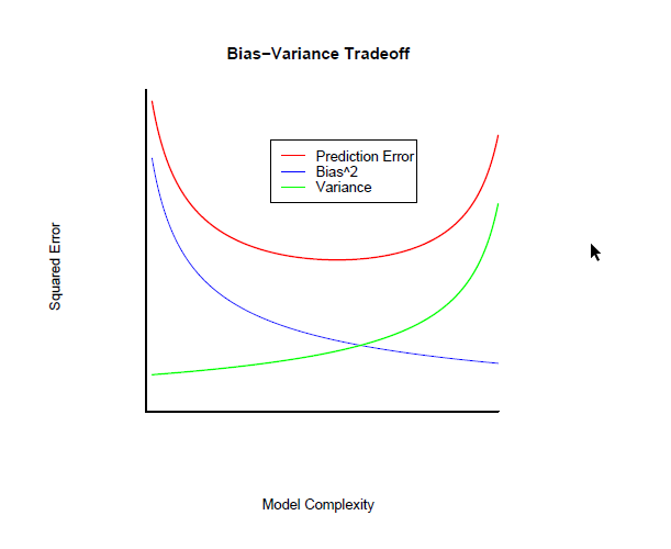
Hence, introducing a little bias in the estimators might lead to a substantial decrease in variance, and hence to a substantial decrease in PE. The idea is then not to let the \(\hat{\beta}_j\) take too large values in order to avoid too large variances. To control the variance, the slope coefficients are regularized in that a constraint is added to the optimization problem (e.g. LS) that controls how large the coefficients can be.

4.2 Ridge regression

The first proposed regularization method is the ridge constraint (or Tikhonov regularization https://en.wikipedia.org/wiki/Tikhonov_regularization), which amounts to set the constraint \(\sum_{i=1}^p\beta_j^2<t_{\lambda}\). In terms of optimization, for a given value of \(\lambda\), the ridge estimator \(\hat{\boldsymbol{\beta}}(\lambda)\) is given by \[\begin{equation} \hat{\boldsymbol{\beta}}(\lambda)=\mbox{argmin}_{\boldsymbol{\beta}}\left\Vert\mathbf{y}-\mathbf{X}\boldsymbol{\beta}\right\Vert^2-\lambda\Vert\boldsymbol{\beta}\Vert^2 \end{equation}\] The solution is \[\begin{eqnarray} \hat{\boldsymbol{\beta}}(\lambda)&=&\left(\mathbf{X}^T\mathbf{X}+\lambda\mathbf{I}\right)^{-1}\mathbf{X}^T\mathbf{y}\\ &=& \left(\mathbf{X}^T\mathbf{X}+\lambda\mathbf{I}\right)^{-1}\left(\mathbf{X}^T\mathbf{X}\right)\hat{\boldsymbol{\beta}}_{LS} \end{eqnarray}\]

Hence, the variance of \(\hat{\boldsymbol{\beta}}_{LS}\) is shrunk by an amount of \(\left(\mathbf{X}^T\mathbf{X}+\lambda\mathbf{I}\right)^{-1}\left(\mathbf{X}^T\mathbf{X}\right)\) which depends on \(\lambda\). With \(\lambda=0\), there is no shrinkage and \(\hat{\boldsymbol{\beta}}(0)=\hat{\boldsymbol{\beta}}_{LS}\), while when \(\lambda\rightarrow\infty\), \(\hat{\boldsymbol{\beta}}(\lambda)\rightarrow\mbox{0}\), the maximal shinkage.

Reported from Efron and Hastie (2016), Section 7.2: Ridge regression applied to the diabetes data

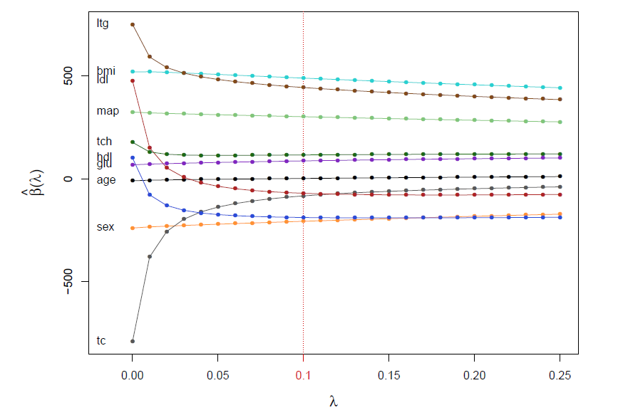
Ridge estimators have lower variance the the LS, but this does not guarantee that the corresponding predictions \(\hat{\boldsymbol{\mu}}\left(\lambda\right)=\mathbf{X}\hat{\boldsymbol{\beta}}(\lambda)\) are more accurate than the ones obtained by the LS \(\hat{\boldsymbol{\mu}}(0)=\mathbf{X}\hat{\boldsymbol{\beta}}(0)\), since \(\hat{\boldsymbol{\beta}}(\lambda)\) is biased towards \(\mathbf{0}\). However, in high dimensions, the prior belief is that most of the \(\beta_j\) lie near zero, and biasing the LS estimator toward zero then becomes a necessity.

Another notable advantage of the ridge estimator is that the inclusion of \(\lambda\) makes the optimization problem solvable even if \(\mathbf{X}^T\mathbf{X}\) is not invertible (e.g. \(\mathbf{X}\) is not of full rank when \(p>n\)). This was the original motivation for ridge regression as proposed by Hoerl and Kennard (1970) who also recommended to select \(\lambda\) graphically. Standard practice now is to use (10-fold) cross-validation.

Exercise
- Use the function glmnet() to perform a Ridge regression on Zambia dataset, plot the values as a function of \(\lambda\) and comment on the results.
- Use the function cv.glmnet() to perform model selection based on 10-fold Cross Validation (i.e. method to select the \(\lambda\) parameter), plot the results and comment the graph that you obtain. Which values of \(\lambda\) are shown by default?
- Use the function predict() to retrieve the final model estimates and perform a simple linear model on the same covariates, what can you conclude?

4.3 The lasso estimator

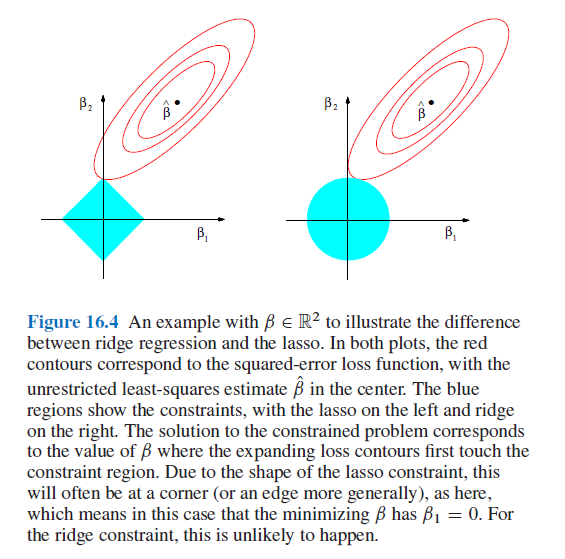
Instead of regularizing the estimator using \(\sum_{i=1}^p\beta_j^2=\Vert\boldsymbol{\beta}\Vert^2<t_{\lambda}\), one could use other \(l_q\)-norms, i.e. \(\Vert\boldsymbol{\beta}\Vert_{q}=\sum_{i=1}^p\vert\beta_j\vert^{q}<t_{\lambda}\). In particular, when \(q=0\), we have \(\Vert\boldsymbol{\beta}\Vert_{0}=\sum_{i=1}^p\vert\beta_j\vert^{0}<t_{\lambda}\) with, by definition, \(\sum_{i=1}^p\vert\beta_j\vert^{0}=\sum_{i=1}^pI\left(\beta_j\neq 0\right)\), the number of slope coefficients different from \(0\), and hence corresponds to subset selection.

Tibshirani (1996) proposed to use \(q=1\) leading to the very famous lasso estimator. The great advantage of the lasso, on top of the fact that the resulting optimization problem \[\begin{equation} \hat{\boldsymbol{\beta}}(\lambda)=\mbox{argmin}_{\boldsymbol{\beta}}\left\Vert\mathbf{y}-\mathbf{X}\boldsymbol{\beta}\right\Vert^2-\lambda\Vert\boldsymbol{\beta}\Vert_1 \end{equation}\]

is convex (since both the loss \(\left\Vert\mathbf{y}-\mathbf{X}\boldsymbol{\beta}\right\Vert^2\) and the constraint \(\Vert\boldsymbol{\beta}\Vert_1=\sum_{j=1}^p\vert\beta_j\vert\) are convex in \(\boldsymbol{\beta}\)), is that the shrinking forces a set of \(\beta_j\) to exactly \(0\). Hence, the lasso estimator provides simultaneously a regularized estimator and model (subset) selection.

Reported from Efron and Hastie (2016), Section 16.2

As for the ridge estimator, \(\lambda\) needs to be chosen and, for model selection purposes (or out-of-sample prediction error optimization), a criteria that assesses the model validity can be used. The most comon choices are the \(C_p\) and 10-fold CV. Practically, for well chosen values of \(\lambda\), \(\hat{\boldsymbol{\beta}}(\lambda)\) and the corresponding model validity criterion are computed. \(\lambda\) is chosen as to optimize (minimize) the later.

To compute the entire lasso path (i.e. for all values of \(\lambda\) that add one \(\beta_j\neq 0\) at each step), Efron et al. (2004) propose the Least Angle Regression algorithm (LARS), which is based on correlations between the covariates to enter and the residuals from the previous fit. LARS is introduced as a more democratic version of forward stepwise regression. Indeed, while forward stepwise regression builds a model sequentially, adding one variable at a time and updating the LS estimator to include all the active variables, the LARS only enters as much of a covariate as it deserves. At the first step it identifies the variable most correlated with the response, and moves the coefficient of this variable continuously toward (not fully) its LS estimate. The residuals are updated and this causes the correlations with other variables to evolve. As soon as another variable reaches the same correlation with the residual as the ones in the active set, this variable then joins the active set.

Reported from Hastie, Tibshirani, and Friedman (2009), Section 3.4. Note that \(\langle \mbox{x}_j,\mathbf{r}\rangle= \mbox{x}_j^T\mathbf{r}\).

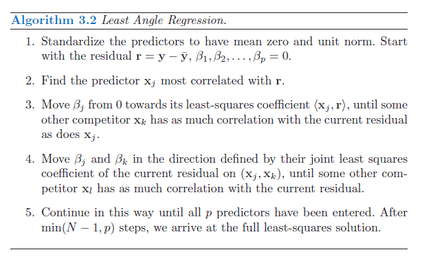
In step 3 and 4, the values of the slopes in the active set, say \(\mathcal{A}\), are augmented as \(\boldsymbol{\beta}_{\mathcal{A}}(\epsilon)=\boldsymbol{\beta}_{\mathcal{A}}+\epsilon\cdot\delta_{\mathcal{A}}\) for small values of \(\epsilon\), with \(\delta_{\mathcal{A}}=\left(\mathbf{X}^T_{\mathcal{A}}\mathbf{X}_{\mathcal{A}}\right)^{-1}\mathbf{X}^T_{\mathcal{A}}\mathbf{r}_{\mathcal{A}}\), \(\mathbf{r}_{\mathcal{A}}=\mathbf{y}-\mathbf{X}_{\mathcal{A}}\boldsymbol{\beta}_{\mathcal{A}}\).

The LARS bears very close similarities with forward stagewise regression (see Hastie et al. (2007), Tibshirani (2015) and Efron and Hastie (2016), Section 16.4). Hence, if the covariates are correlated, the lasso path might not produce the suitable model selection path (risk of overfitting).

Exercise
- Use the function glmnet() to perform a lasso on Zambia dataset, plot the values as a function of \(\lambda\) and comment on the results.
- Use the function cv.glmnet() to perform model selection based on 10-fold Cross Validation (i.e. method to select the \(\lambda\) parameter), plot the results and comment the graph that you obtain. Which values of \(\lambda\) are shown by default? What can you conclude on the choice of \(\lambda\) in terms of model selection?
- Use the function predict() to retrieve the final model chosen by 10-fold CV (given lasso ordering) and perform a linear model on the covariates present in the final model. What can you conclude observing the estimates?

4.4 Alternative penalized regression methods

4.4.1 The adaptive and relaxed lasso

Because the lasso finds a suitable compromise between estimation bias and variance, the price to pay is that it generally provides (asymptotically) biased slope estimators. It can be shown that the bias is larger for (true) large slope coefficients (in absolute value). Ideally then, one should consider, instead of the lasso penalty \(\lambda\Vert\boldsymbol{\beta}\Vert_1\), more generally \(\sum_{j=1}^p\lambda_j\vert\beta_j\vert\). Zou (2006) propose the adaptive lasso with \(\lambda_j=\lambda w_j^{\gamma}\) and \[\begin{equation} w_j^{\gamma}=\left\vert \hat{\beta}_{j}^{(LS)}\right\vert^{-\gamma}, \; \gamma>0 \end{equation}\]

Hence, \(w_j\) assigns smaller weights to larger slope coefficients, and when \(\hat{\beta}_{j}^{(LS)}\rightarrow 0\), \(w_j \rightarrow \infty\) so that the adaptive lasso estimate \(\hat{\beta}_j \rightarrow 0\). Actually, \(\hat{\boldsymbol{\beta}}^{(LS)}\) can be replaced by any (\(\sqrt{n}\)) consistent estimator of \(\boldsymbol{\beta}\). In practice, when \(p>n\), the ridge estimator is a suitable candidate.

The corresponding optimization problem is \[\begin{equation} \hat{\boldsymbol{\beta}}(\lambda,\gamma)=\mbox{argmin}_{\boldsymbol{\beta}}\left\Vert\mathbf{y}-\mathbf{X}\boldsymbol{\beta}\right\Vert^2-\lambda\sum_{j=1}^pw_j^{\gamma}\vert\beta_j\vert \end{equation}\] and remains a convex optimization problem. Actually, the LARS algorithm can be used to obtain the adaptive losso path, by applying it to the scaled covariates \(\tilde{\mathbf{x}}_j=\mathbf{x}_j/w_j^{\gamma}\). Namely, let \(\tilde{\mathbf{X}}=\left[\tilde{\mathbf{x}}_j\right]_{j=1,\ldots,p}\) and \[\begin{equation} \tilde{\boldsymbol{\beta}}(\lambda)=\mbox{argmin}_{\boldsymbol{\beta}}\left\Vert\mathbf{y}-\tilde{\mathbf{X}}\boldsymbol{\beta}\right\Vert^2-\lambda\Vert\boldsymbol{\beta}\Vert_1 \end{equation}\]

the adpative lasso estimator is \(\left[\hat{\beta}_j(\lambda,\gamma)\right]_{j=1,\ldots,p}\) with \(\hat{\beta}_j(\lambda,\gamma)=\tilde{\beta}_j(\lambda)/w_j^{\gamma}\).

As with the lasso, the question of the choice of the tunning parameters is crucial. Since there are two, ideally all combiations of \((\lambda,\gamma)\) should be evaluated. Hence, for a given \(\gamma\), \(\lambda\) is optimized using an out-of-sample validation measure such as 10-fold CV or the \(C_p\) to get \(\lambda_{\gamma}\) and in a second layer, \(\gamma\) is also optimized (actually \((\gamma,\lambda_{\gamma})\) is optimized in \(\gamma\)) again using an out-of-sample validation measure such as 10-fold CV or the \(C_p\). The choice for the latter does not have to be the same for \(\lambda\) and \(\gamma\).

The adaptive lasso is a two-stage approach, with at the first stage a chosen initial estimator which produces a single set of weights \(w_j^{\gamma}\) which are held constant (for fixed \(\gamma\)) across all values of \(\lambda\). An alternative approach, known as a pathwise approach is to let the weights change with \(\lambda\): \(w_j^{\gamma\lambda}:=w_j^{\gamma\lambda}\left(\hat{\beta}_j\right)\). A notable example is the relaxed lasso of Meinshausen (2007) which, for \(\lambda\geq 0\) and \(0<\phi\leq 1\) is given by \[\begin{equation} \hat{\boldsymbol{\beta}}(\lambda,\phi)=\mbox{argmin}_{\boldsymbol{\beta}}\left\Vert\mathbf{y}-\sum_{j=1}^p\mathbf{x}_j{\beta}_jI\left(j\in \mathcal{A}_{\lambda}\right)\right\Vert^2-\phi\lambda\Vert\boldsymbol{\beta}\Vert_1 \end{equation}\]

with \(\mathcal{A}_{\lambda}\) the set of indicators of the covariates in the active set produced by the corresponding \(\lambda\). The later hence controls the variable selection part, as in the lasso, while the relaxation parameter \(\phi\) controls the shrinkage of coefficients. If \(\phi= 1\), the lasso and relaxed lasso estimators are identical, and for \(\phi<1\), the shrinkage of coefficients in the selected model is reduced compared to the lasso. When \(\phi\rightarrow 0\), \(\hat{\beta}_j(\lambda,\phi)\rightarrow\hat{\beta}_j^{(LS/\mathcal{A}_{\lambda})}\), where the \(\hat{\beta}_j^{(LS/\mathcal{A}_{\lambda})}\) is the LS obtained on the subset \(\mathcal{A}_{\lambda}\). Note that if \(\phi=0\) one gets the LS on the full model (the effect of \(\lambda\) as variable selection tunning parameters disappears).

To obtain the relaxed lasso solutions, one first sets \(\phi=1\) and obtains the lasso path, then for each submodel of the lasso path, the LARS algorithm is run by varying the penalty \(\phi\lambda\) through \(\phi\). There is in general no need to do the full LARS in the second stage so the compuation can be nearly as fast as a for the lasso. Again, the tunning parameters \((\lambda,\phi)\) can be determined by 10-fold CV.

4.4.2 The elastic net

When there is strong correlation among the covariates, the lasso estimator will somehow arbitrarily choose among a set of strong but correlated variables. The ridge penalty, on the other hand, tends to shrink the coefficients of correlated variables toward each other. The elastic net penalty proposed by Zou and Hastie (2005) is a comprimise between the lasso and ridge regression and the estimators are the solution of the optimization problem \[\begin{equation} \hat{\boldsymbol{\beta}}(\lambda)=\mbox{argmin}_{\boldsymbol{\beta}}\left\Vert\mathbf{y}-\mathbf{X}\boldsymbol{\beta}\right\Vert^2-\alpha\lambda\Vert\boldsymbol{\beta}\Vert_1-\frac{1}{2}(1-\alpha)\lambda\Vert\boldsymbol{\beta}\Vert^2 \end{equation}\]

The elastic net solution contains in general more active covariates with smaller coefficients. The introduction of the ridge penalty has the effect of reducing the variance of lasso estimates at the cost of further increasing their bias. Adding a ridge penalty is not always universally benefficial, as the bias can dominate the variance. However, since like ridge regression, the elastic net shrinks the coefficients of correlated variables toward each other, it tends to select correlated variables in groups, which might be an advantage in for example biological studies.

4.4.3 The nonnegative garrote

Based on the argument that shrinking decreases the estimation/prediction variance, Breiman (1995) proposes to directly define shrunk estimators as \[\begin{equation} \hat{\beta}_j(\lambda)=u_j(\lambda)\hat{\beta}_j^{(LS)} \end{equation}\] with shrinking factors (or garrote) \(\mathbf{u}(\lambda)=[u_j(\lambda)]_{j=1,\ldots,p}\) obtained as \[\begin{eqnarray} & \mathbf{u}(\lambda)=\mbox{argmin}_{\mathbf{u}=[u_1\ldots u_p]}\left\Vert\mathbf{y}-\mathbf{X}\mathbf{B}\mathbf{u}\right\Vert^2-2\lambda\sum_{j=1}^pu_j \\ & \mbox{s.t. } u_j\geq 0 \forall j \end{eqnarray}\]

with \(\mathbf{B}=\mbox{diag}\left(\hat{\beta}_j^{(LS)}\right)\). The penalty corresponds to the constraint \(\sum_{j=1}^pu_j\leq t_{\lambda}\). For sufficiently large \(\lambda\) some of the \(u_j\) will be set to 0, so that the nonnegative garrote estimator performs simultaneously shinking and subset selection.

Yuan and Lin (2007) propose to use a slightly modified version of the LARS to obtain the solution path for the nonnegative garrote estimators. Indeed, since \(\mathbf{B}\) is provided in an initial stage, then one can use the LARS (adapted to the positivity constraints) in which \(\mathbf{X}\rightarrow \tilde{\mathbf{X}}=\mathbf{X}\mathbf{B}\) and \(\boldsymbol{\beta}\rightarrow \mathbf{u}\), \(\lambda\rightarrow 2\lambda\).

The adaptive lasso with \(\gamma=1\) corresponds to the nonnegative garrote (when adding the positivity constraints). Indeed, we have \(u_j=\vert\beta_j\vert/\vert\beta_j^{(LS)}\vert\) with the constraints \(\beta_j\beta_j^{(LS)}\geq 0\), \(\forall j\), so that \(\mathbf{X}\mathbf{B}\mathbf{u}=\mathbf{X}\boldsymbol{\beta}\).

Given the form of the nonnegation garrote estimator \(\hat{\boldsymbol{\beta}}(\lambda)=\left[\hat{\beta}_j(\lambda)\right]_{j=1,\ldots,p}\), it is straightforward to derive Efron's covariance penalty estimator of out-of-sample prediction error. Indeed, \(\hat{\mathbf{y}}=\mathbf{X}\mathbf{B}\mathbf{u}=\mathbf{X}\mathbf{U}\hat{\boldsymbol{\beta}}^{(LS)}=\mathbf{X}\mathbf{U}\left(\mathbf{X}^T\mathbf{X}\right)^{-1}\mathbf{X}^T\mathbf{y}\), with \(\mathbf{U}=\mbox{diag}\left(u_j\right)\), and \[\begin{equation} \mbox{tr}\left(\mbox{cov}(\hat{\mathbf{Y}},\mathbf{Y})\right)= \sigma^2\mbox{tr}\left(\mathbf{X}\mathbf{U}\left(\mathbf{X}^T\mathbf{X}\right)^{-1}\mathbf{X}^T\right)=\sigma^2\mbox{tr}\left(\mathbf{U}\right)=\sigma^2\sum_{j=1}^pu_j; \end{equation}\]

by using the cyclic property of the trace operator (see also Xiong (2010)). Therefore, one can determine the \(u_j\) by minimizing the estimated out-of-sample prediction error, i.e. \(\mbox{min}_{\mathbf{u}} \Vert \mathbf{y}−\mathbf{X}\mathbf{U}\hat{\boldsymbol{\beta}}^{(LS)}\Vert+2\sigma^2 \sum_{j=1}^pu_j\), s.t. \(u_j \geq 0\), \(\forall j\), which yields the nonnegative garrote estimator with tuning parameter \(\lambda = \sigma^2\). In practice, \(\sigma^2\) is replaced by a consistent estimator \(\hat{\sigma}^2\); for a review, see e.g. Reid, Tibshirani, and Friedman (2016).

4.4.4 Non convex penalties

The adaptive lasso consists of a two-stage approach involving an initial estimator to reduce bias for large regression coefficients. An alternative single-stage approach is to use a penalty that tapers off as \(\beta_j\) becomes larger in absolute value. Unlike the absolute value penalty employed by the lasso, a tapering penalty function cannot be convex. Such functions are often referred to as folded concave, in that it is symmetric around \(\beta_j=0\). The penalty function, say \(\sum_{j=1}^pP(\beta_j\vert \lambda,\gamma)\), then involves a tuning parameter \(\gamma\) that controls the concavity of the penalty (i.e., how rapidly the penalty tapers off). Using a penalty that does not taper off (e.g. the lasso penalty) is called soft thresholding, while using subset (forward stepwise) selection (i.e. the \(l_0\) norm) is called hard thresholding.

A popular penalty is the smoothly clipped absolute deviations (SCAD) penalty of Fan and Li (2001), given by \[\begin{eqnarray} P(\beta_j\vert \lambda,\gamma)=\left\{\begin{array}{ll} \lambda\vert\beta_j\vert & \mbox{if } \;\vert\beta_j\vert\leq\lambda \\ \frac{2\gamma\lambda\vert\beta_j\vert-\beta_j^2-\lambda^2}{2(\gamma-1)} & \mbox{if } \;\lambda<\vert\beta_j\vert\leq\gamma\lambda \\ \frac{\lambda^2(\gamma+1)}{2} & \mbox{if } \;\vert\beta_j\vert>\gamma\lambda \end{array} \right. \end{eqnarray}\] for \(\gamma>2\). The SCAD coincides with the lasso until \(\vert\beta_j\vert=\lambda\), then smoothly transits to a quadratic function until \(\vert\beta_j\vert = \gamma\lambda\), after which it remains constant. The derivative of the SCAD penalty is \[\begin{eqnarray} \frac{\partial}{\partial\beta_j}P(\beta_j\vert \lambda,\gamma)=\left\{\begin{array}{ll} \lambda & \mbox{if } \;\vert\beta_j\vert\leq\lambda \\ \frac{\gamma\lambda-\vert\beta_j\vert}{\gamma-1} & \mbox{if } \;\lambda<\vert\beta_j\vert\leq\gamma\lambda \\ 0 & \mbox{if } \;\vert\beta_j\vert>\gamma\lambda \end{array} \right. \end{eqnarray}\]

The SCAD penalty retains the penalization rate (and bias) of the lasso for small coefficients, but continuously relaxes the rate of penalization (and bias) as the absolute value of the coefficient increases. Hence the overall bias is reduced.

Another population non convex penalty has been proposed by Zhang (2010) as the Minimax Concave Penalty (MCP), given by \[\begin{eqnarray} P(\beta_j\vert \lambda,\gamma)=\left\{\begin{array}{ll} \lambda\vert\beta_j\vert - \frac{\beta_j^2}{2\gamma}& \mbox{if } \;\vert\beta_j\vert\leq \gamma\lambda \\ \frac{\lambda^2\gamma}{2} & \mbox{if } \;\vert\beta_j\vert>\gamma\lambda \end{array} \right. \end{eqnarray}\] for \(\gamma>1\). Its derivative is \[\begin{eqnarray} \frac{\partial}{\partial\beta_j}P(\beta_j\vert \lambda,\gamma)=\left\{\begin{array}{ll} \mbox{sign}\left(\beta_j\right)\left(\lambda - \frac{\vert\beta_j\vert}{\gamma}\right)& \mbox{if } \;\vert\beta_j\vert\leq\gamma\lambda \\ 0 & \mbox{if } \;\vert\beta_j\vert>\gamma\lambda \end{array} \right. \end{eqnarray}\]

As with the SCAD, the MCP starts out by applying the same rate of penalization as the lasso, then smoothly relaxes the rate down to zero as the absolute value of the coefficient increases. It does however so immediately while with SCAD the rate remains flat for a while before decreasing.

Reported from Zhang (2010), Figure 1. Penalty functions (right panel) and their derivatives (left panel) as a function of \(\vert\beta_j\vert\), for the lasso (\(t\)), SCAD and MCP with \(\gamma=2.5\).

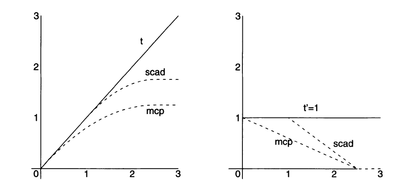
As \(\gamma\rightarrow\infty\), both the MCP and SCAD penalties converge to the \(l_1\) penalty. As \(\gamma\) approaches its minimum value, the bias is minimized. The price to pay is the instability of the resulting MCP and SCAD estimators, in the sense that as the penalty becomes more concave (i.e. for smaller \(\gamma\)), there is a greater chance for the optimization problem to admit multiple local minima.

Among others, Zhang (2010) and Breheny and Huang (2011) propose algorithms to find the SCAD and MCP estimates, or more generally, penalized regression estimators with non convex penalties. Moreover, as with the elastic net, one can add a ridge penalty to nonconvex penalties such as MCP and SCAD.

Exercise
After having read the documentation of the R package ncvreg and installed it, perform the following steps:

1. Fix the generating vector \(\boldsymbol{\beta}=(4,2,-4,-2,0,0,\ldots,0)\) and set the seed equal to 11 (i.e. set.seed(11)).
   

2. Generate from a MVN (multivariate normal) a matrix \(\mathbf{X_{n*p}}\) with \(n = 200\) and \(p = 1000\). You can choose the location vector as you wish but set the scale matrix with an autoregressive form \(\boldsymbol{\Sigma}=[\sigma_{lm}]_{l,m=1,\ldots,p}\) with \(\sigma_{lm} = \rho^{\mid l - m\mid}\). 

3. For each \(\boldsymbol{\rho} = [0 \; 0.2 \; 0.5]\) generate \(\mathbf{\hat{y}}\) thanks to the relation \(\mathbf{y} = \mathbf{X_{n*p}} \; \boldsymbol{\beta} + \boldsymbol{\epsilon}\) where \(\epsilon_{i}\) is a standard normal. Suppose for simplicity that the errors are uncorrelated.
   

4. Compare the solution paths (graphically as a function of \(\lambda\)) for the lasso, SCAD and MCP by fixing several values for \(\gamma\) (choose e.g. \(\gamma=(1.5, 2, 3, 3.7, 5)\)) for each value of \(\rho\) indicated at point c.

References

Breheny, P., and J. Huang. 2011. “Coordinate Descent Algorithms for Nonconvex Penalized Regression, with Applications to Biological Feature Selection.” The Annals of Applied Statistics 5: 232–53.

Breiman, L. 1995. “Better Subset Regression Using the Nonnegative Garrote.” Technometrics 37: 373–84.

Efron, B., and T. Hastie. 2016. Computer Age Statistical Inference: Algorithms, Evidence, and Data Science. Cambridge University Press.

Efron, B., T. Hastie, I. Johnstone, and R. Tibshirani. 2004. “Least Angle Regression (with Discussion).” Annals of Statistics 32: 407–99.

Fan, J., and R. Li. 2001. “Variable Selection via Nonconcave Penalized Likelihood and Its Oracle Properties.” Journal of the American Statistical Association 96 (456). Taylor & Francis: 1348–60.

Hastie, T., J. Taylor, R. Tibshirani, and G. Walther. 2007. “Forward Stagewise Regression and the Monotone Lasso.” Electronic Journal of Statistics 1: 1–29.

Hastie, Trevor, Tibshirani Robert, and Jerome Friedman. 2009. The Elements of Statistical Learning: Data Mining, Inference, and Prediction. Second Edition. Springer Series in Statistics. Springer.

Hoerl, A. E., and R. Kennard. 1970. “Ridge Regression: Biased Estimation for Nonorthogonal Problems.” Technometrics 12: 55–67.

James, W., and C. Stein. 1961. “Estimation with Quadratic Loss.” In Proc. 4th Berkeley Symposium on Mathematical Statistics and Probability, Vol. I, 361–79. University of California Press.

Meinshausen, N. 2007. “Relaxed Lasso.” Computational Statistics and Data Analysis 52: 374–93.

Reid, S., R. Tibshirani, and J. Friedman. 2016. “A Study of Error Variance Eestimation in Lasso Regression.” Statistica Sinica 26: 35–67.

Tibshirani, R. 1996. “Regression Shrinkage and Selection via the Lasso.” Jrssb 58: 267–88.

Tibshirani, R. J. 2015. “A General Framework for Fast Stagewise Algorithms.” Journal of Machine Learning Research 16: 2543–88.

Xiong, S. 2010. “Some Notes on the Nonnegative Garrote.” Technometrics 52 (3): 349–61.

Yuan, M., and Yi Lin. 2007. “On the Non-Negative Garrotte Estimator.” Journal of the Royal Statististical Sociaty, Series B 69: 143–61.

Zhang, C.-H. 2010. “Nearly Unbiased Variable Selection Under Minimax Concave Penalty.” The Annals of Statistics 38: 894–942.

Zou, H. 2006. “The Adaptive Lasso and Its Oracle Properties.” Journal of the American Statistical Association 101: 1418–29.

Zou, H., and T. Hastie. 2005. “Regularization and Variable Selection via the Elastic Net.” Journal of the Royal Statistical Society: Series B 67 (2). Wiley Online Library: 301–20.